Friday, 15 December 2017

MARKET EQUILIBRIUM AND GOVERNMENT INTERVENTION

MARKET EQUILIBRIUM

DEFINITION
The quantity in which producers are willing to produce and the consumers are willing and able to purchase.

 QUANTITY DEMANDED = QUANTITY SUPPLIED 

 
DETERMINATION OF EQUILIBRIUM PRICE AND QUANTITY
  1. From demand and supply schedules
  2.  From demand and supply curves
 Image result 
DEFINITION OF GOVERNMENT INTERVENTION
The imposition of certain directives by the government,which interferes with the market mechanism.

TYPES OF INTERVENTION
  1. Price control(price floor or minimum price and price ceiling or maximum price)
  2. Indirect tax and subsidy
PRICE CONTROL  
a)Minimum price(price floor)
  • imposed by the government when market price is extremely low
  • Where government help push up the price(agricultural products)
  • At minimum price,supply exceeds demand:therefore,its creates SURPLUS. 
      Image result for SURPLUS 

ADVANTAGES 
=Higher income for FARMERS 

DISADVANTAGES
  1. Consumers have to pay higher price
  2. The problem of surplus.Government has to buy the excess stock by using taxpayers money
  3. The excess stock has to be disposed-causes wastage.
b)Maximum price(price ceiling)
  • imposed by the government when market price is exorbitantly high
  • usually imposed during inflation or war
  • at maximum price,demand exceeds supply:therefore,it creates SHORTAGE.   
 Image result for shortage


ADVANTAGES
Consumers pay lower price


DISADVANTAGES
  1. Due to the problem of shortage,people are willing to pay higher price.This encourages black market and smuggling activities.
  2. Since limited supply,government has to ratio or redistribute
  3. Encourages exploitation by the producers.
     Image result for shortage and surplus


 TAXES
 Image result for gst
DIRECT TAX
Imposed directly on to a person(income tax,company tax).

INDIRECT TAX
Imposed on an entity but that entity can shift the burden of paying tax to someone else(sales tax,import tax).

EFFECTS OF IMPOSING INDIRECT TAXES ON GOODS
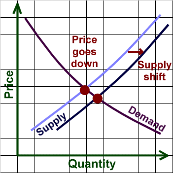
 The imposition of indirect tax will cause the producer to reduce supply.Therefore,supply curve will shift to the left(Supply without tax -->Supply with tax). As a result,price goes up and quantity reduced.
    
Image result for taxes graph

Wednesday, 13 December 2017

Elasticity

Image result for formula elasticity of demand


FORMULA


DEGREE OF PRICE ELASTICITY OF SUPPLY

DEGREE
DESCRIPTION
VALUE OF COEFFICIENT
SLOPE OF SUPPLY CURVE
ELASTIC
%CHANGE Qs > %CHANGE P
SUPPLY ELASTICITY > 1
Related image
INELASTIC
%CHANGE Qs < %CHANGE P
SUPPLY ELASTICITY < 1
Image result for formula elasticity of supply elastic
UNITARY
%CHANGE Qs = %CHANGE P
SUPPLY ELASTICITY = 1
Image result for formula elasticity of supply unitary
PERFECTLY ELASTIC
AT LEVEL P,Qs is infinity
SUPPLY ELASTICITY = INFINITY
Image result for formula elasticity of supply unitary

PERFECTLY INELASTIC
NO CHANGE IN Qs ALTHOUGH P CHANGES
SUPPLY ELASTICITY = 0
Image result for formula elasticity of supply unitary


example for Tesco bread

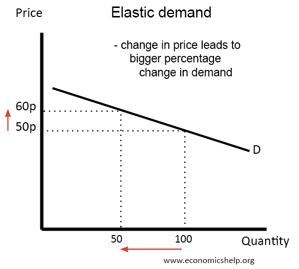
price-elastic-demand


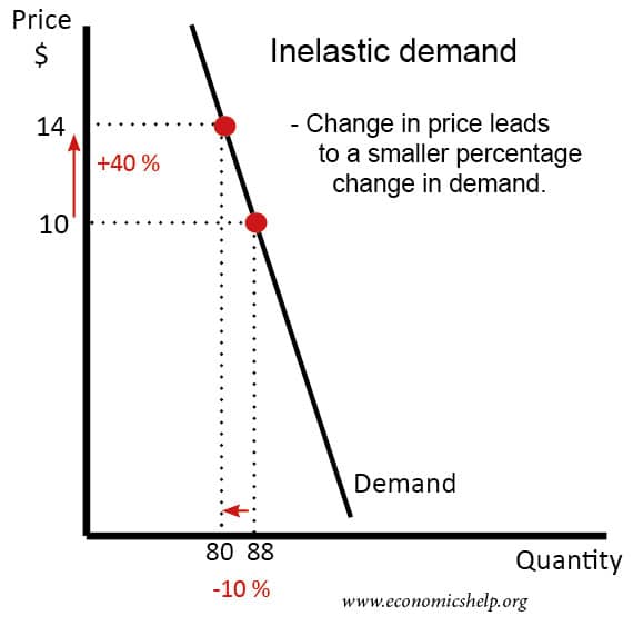
inelastic demand

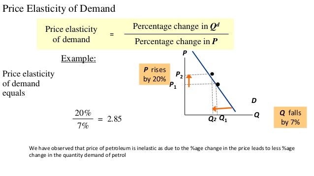
  • for petrol


 petrol has few alternatives because people with a car need to buy petrol. For many driving is a necessity. There are weak substitutes, such as train, walking and the bus. But, generally, if the price of petrol goes up, demand proves very inelastic.


elasticity of supply

Image result for formula elasticity of supply
Given the following data for the supply and demand of movie tickets, calculate the price elasticity of supply when the price changes from $9.00 to $10.00.
Price Elasticity of Supply Example Problem
We know that the original price is $9 and the new price is $10, so we have Price (Old) =$9 and Price (New) = $10. From the chart, we see that the quantity supplied when the price is $9 is 75 and when the price is $10 is 105.
So we have:
Price (Old) = $9
Price (New) = $10
Quantity Supplied (Old) = 75
Quantity Supplied (New) = 105


Monday, 11 December 2017

theory elasticity of demand and supply

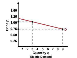
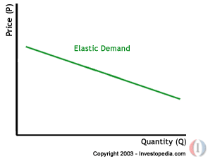
Elasticity = (% change in quantity / % change in price)
If the elasticity is greater than or equal to 1, the curve is considered to be elastic. If it is less than one, the curve is said to be inelastic.

economics12.gif

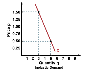
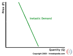
Meanwhile, inelastic demand can be represented with a much steeper curve: large changes in price barely affect the quantity demanded.
Related image


Related image
economics13.gifMeanwhile, inelastic demand can be represented with a much steeper curve: large changes in price barely affect the quantity demanded


Related image


demand and supply

THE LAW OF DEMAND


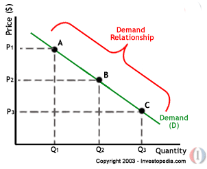
economics3.gifA, B and C are points on the demand curve. Each point on the curve reflects a direct correlation between quantity demanded (Q) and price (P). So, at point A, the quantity demanded will be Q1 and the price will be P1, and so on. The demand relationship curve illustrates the negative relationship between price and quantity demanded. The higher the price of a good the lower the quantity demanded (A), and the lower the price, the more the good will be in demand (C).

Read more: Law of Supply and Demand: Basic Economics https://www.investopedia.com/university/economics/economics3.asp#ixzz50xuLjTK5 


/


cow.jpg

Example

Here's a real life example using ground beef. The USDA has calculated that the demand elasticity for beef is -0.621. That means that, as the price rise 1.0 percent, the quantity demanded fall 0.621 percent. This is fairly inelastic because the quantity doesn't fall as much as the price rose.
(Source:  "Price Elasticity Estimates," U.S. Department of Agriculture.) 
In 2014, the price of ground beef rose dramatically, thanks to two droughts in a row. The first was in 2012, driving up food prices and forcing cattle ranchers to slaughter their cows to prevent them from starving. In 2014, another drought drove grain prices up again. Ranchers hadn't yet rebuilt their herds, so prices for beef simply rose. For more, see Why Are Food Prices So High?  (Source: "Average Food and Energy Prices," Bureau of Labor Statistics.)
For this example, let's say a family of four bought 10 pounds of ground beef in January to make hamburgers, meat loaf and chili. All other things being equal, here's the demand schedule showing how they would reduce the quantity bought by 0.621 percent for every 1.0 percent the price actually rose.
Month in 2014Price/lb.Quantity (in lbs.)
Jan  $3.467   10.000
Feb  $3.555     9.842
Mar  $3.698     9.597
Apr  $3.808     9.419
May  $3.856     9.346
Jun  $3.880     9.309
Jul  $3.884     9.303
Aug  $4.013     9.112
Sep  $4.096     8.995
Oct  $4.454     8.506
Although prices rose 28.4 percent, the quantity bought only fell 14.9 percent because demand is fairly inelastic. These quantities assume all other determinants of demand remain the same.
 If the determinants of demand other than price change, it shifts the entire demand curve. That's because a whole new demand schedule will need to be created, to show the new relationship between price and quantity. For more, see Demand Curve Shift.


economics4.gif

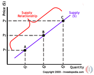
A, B and C are points on the supply curve. Each point on the curve reflects a direct correlation between quantity supplied (Q) and price (P). At point B, the quantity supplied will be Q2 and the price will be P2, and so on. (To learn how economic factors are used in currency trading, read Forex Walkthrough: Economics.)

Read more: Law of Supply and Demand: Basic Economics https://www.investopedia.com/university/economics/economics3.asp#ixzz50xwsjZHl
Follow us: Investopedia on Facebook


Example #1: The Price of Oranges In this case we will look at how a change in the supply of oranges changes the price The demand for oranges will stay the same. The demand curve doesn't change. In the first year, the weather is perfect for oranges. Orange farmers have a bumper crop. This increases the supply of oranges. Because there are so many more oranges on the market, the farmers reduce the price of oranges in order to sell


economics5.gif
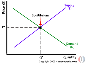
equilibrium occurs at the intersection of the demand and supply curve, which indicates no allocative inefficiency. At this point, the price of the goods will be P* and the quantity will be Q*. These figures are referred to as equilibrium price and quantity.
In the real market place equilibrium can only ever be reached in theory, so the prices of goods and services are constantly changing in relation to fluctuations in demand and supply.